Maintenance Free Operating Period (MFOP)

Maintenance Free Operating Period (MFOP) is a concept pertaining to the maintenance policies for systems that operate in alternating "work-rest" environment. The nature and the durations of cycles can vary, but the bottom line remains the same: the goal is to conduct as much maintenance as possible during the "rest" (recover) phase, and avoid system failures during the "work" phase. A simple example of such cyclical schedule are airline operations: generally, the night is the recovery phase (with the few red-eye exceptions). Military operations is another important example, with the recovery phase usually much longer then a single night.

The following discussion extends the example previously studied across the pond¹. The goal is to explore the implications of different design changes, including redundancies, reconfiguration, and preventive maintenance. The four phases from the original example are retained, however instead of all failures following exponential distributions, Weibull distributions for two components (A and B) are considered. The full set of parameters (which is different from those in [1]) is shown in Table 1. The source XLS file for these parameters can be found here. An APN file can be linked to a corresponding XLS parameter file (the last item under the Parameters menu). After the XLS file is linked, one can change parameters in that file, save the changes, and then click under the same menu in APN on "Update from Linked file" to update parameters in the model.

In order to understand how the APN model for MFOP is constructed, we start with a basic model shown in Figure 1. This model has four components (A,B,C,D as represented by tokens with colors 0,1,2,3, respectively) that sequentially go through four phases with no maintenance. The places shown with slightly thicker lines correspond to the fused places - after four phases are completed (moving from the left to the right), the first phase starts again².

The source file for this APN model can be found here. Note that APN files have extension .apn, but they are effectively XML files, so you browser might simply show the file instead of saving it. If that is the case, simply save the file and use extension .apn. After you run the model (unless you changed the simulation time it is set at 297 (hours) or 36 missions), what can you conclude about the chances of failure? Can you calculate those chances analytically? If yes, how?

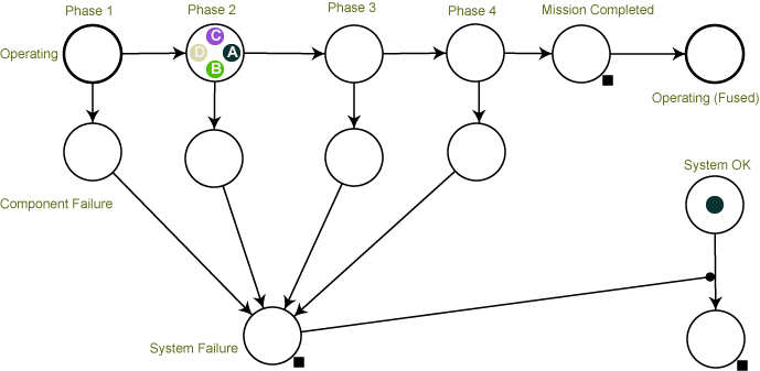
Next, let us introduce the redundancies (described in [1])) as shown in Figure 2. The bottom portion of the model has an additional structure that specifies for each phase which components cause system failure. Enablers (arcs terminated with solid circles) of multiplicity two to ensure that a token moves to the system failure place only if there are two tokens in the corresponding place where an enabler originates. The source file for this APN model can be found here.

After you run the second model, do you see much difference? Here the components that don't cause the failure for a given phase are still operating during that phase (and can fail). Depending on the modeled system, you might want to model a scenario where such components are actually idle during that phase. For example, component C does not contribute to the failure during Phase 1. Double clicking on the corresponding transition, selecting the policy for component C (color 2) shows that it is currently linked to the parameter with the failures for component C. You can uncheck the link box and then select transition type to "None". The resulting model describes a scenario where component C is idle during this phase. Similar changes can be made to other components.

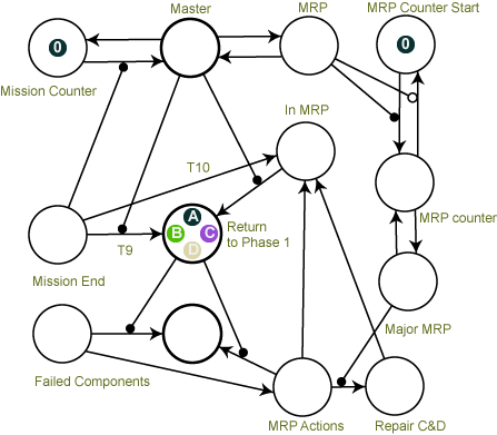
Next, you can explore the models that introduce MFOP, as described in [1]). The source file for this APN model can be found here. The additional portion on the left counts the missions (on the top) and also replaces components as needed. This portion is shown in Figure 3. When a mission is completed the components that have not failed yet arrive to the "Mission End" place. There is at least one of such components (why?), and the enabler connecting this place to the transition from Mission Counter is activated. The token from the Mission Counter place, shown in Figure 3 with label (color) zero, moves to the right into the "Master" place with its color incremented by one. The process is repeated as missions are completed, until the number of missions (reflected in the token's color) reaches the MFOP, then this token moves to the right to the "MRP" (Maintenance Recovery Period). When it happens, the T10 is fired rather than T9 (timing of transitions are selected to ensure that this happens in the abscence of the mission token in the "Master" place). As a result, the tokens from the "Failed Components" move to the "MRP actions" place. There is an additional counter on the right that diffentiates minor and major MRP. When the corresponding token is moved to the "Major MRP" place, the transition from the "MRP Actions" to the "Repair C&" is enabled, and tokens corresponding to those components are moved to the "Repair C&" place. For minor MRP only components A and B are repaired.

Finally, the last source file has the same model, but it resets the age of the Weibull components after each MFOP (equivalent to replacing those components with the new ones). The source file for this APN model can be found here. Which of the changes makes the biggest impact on the risks of failing during the mission? Can you explain this? Changing the model parameters and looking at the redundancy structure provides useful clues.

Another possible extension is related to the possibility of condition-based maintenance for some of the components. A simple way to model this effect is described in 2015 ESREL paper. A similar two-phase transition to failure can be added to the MFOP model described here by changing the color of a component when it moves to the detectable damage (for example, by introducing an additional places on the top of the operation for each phase where the transition to this phase occurs and the token for the corresponding component is returned to the operating place).