One of the distinguishing features of APN is its implementation of the aging token concept. Originally introduced in 2004, aging tokens allow additional flexibility in providing tokens with some memories about their past. As always, there is an issue of a balance between modeling power and simplicity. Token's age is simply a value \(\eta\in \left[0,1\right]\) that represents this past in a simplified fashion. This value affect the firing time of a transition.
Let us consider a situation when there are two tasks needed to be accomplished sequentually within a given amount of time. We will refer collectively to the instance of the problem as a "case" alluding to a workflow problem for specificity. We would like to know whether this could be achieved successfully or not. First, let us look at a model that does not utilize aging tokens.
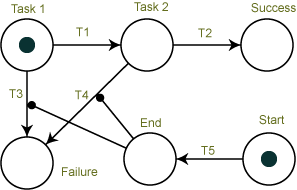
Figure 1: APN model for two sequential tasks without aging
Transition T5 represents a global "clock": when the alotted time expires, the case token in the Start place moves to the End place, which triggers immediate transitions T3 and T4 and forces the case token to move into the Failure place. The source file for this APN model can be found here. While this "global" solution is workable for this simple scenario, there are difficulties in extending its applicability to realistic applications. For example, we might be interested in several cases occuring in parallel, where each instance represented by a case token would need to accomplish two tasks, so the considered network is a fragment of a larger network. In this situation, we would have to enforce some synchronization ensuring that tokens in the Task 1 and Start places arrive at the same time, and would only be able to treat one token at a time in this subnet. To treat multiple cases, we would need multiple subnets each dedicated to a single case at a time.
Let us contrast this with the model that uses aging tokens. Here the T3 transition is selected to be aging for the Task 1 place (in APN software one needs to bring up the place property dialog, and click on aging transition button that enables the selection of the aging transtion). The main idea is that when the first task is completed and the token moves to the Task 2 place, its age is used to ensure that the delay for the T4 transition is adjusted to account for the time spent in the Task 1 place. For deterministic (fixed) delays the interpretation is more straightforward, so we will consider it first (the source file can be found here).
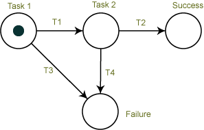
Figure 2: APN model for two sequential tasks with aging
If the aging transition (T3 in this case) has a fixed delay \(\tau\), the age \(\eta\) is simply the fraction of the time it was enabled \(t_e\)for this token as compared to that aging transition delay: \(\eta=t_e/\tau\). For the T4 transition we can select an age-dependent fixed type of a transition with the value the same as T3. There are situations where it is beneficial to have a fixed delay that is independent of the age of the token, and then fixed delay can be selected. Let us consider specific values for the transitions: \(\tau_1=1\) and \(\tau_2=\tau_3=\tau_4=2\). At time \(t=0\), the age of the token is zero. At \(t_1=1\), T1 fires and \(\eta=1/2=0.5\). At this point both T2 and T4 are enabled for this token. T2 is scheduled to fire at time \(t_2=t_1+\tau_2=1+2=3\), while T4 is scheduled to fire at time \(t_3=t_1+(1-\eta)\tau_2=1+2\cdot 0.5=2\), so T4 fires the token first at \(t_3=2\) and the token moves to the Failure place.
Next, let us consider transitions with probabilistic delays that follow a cumulative distribution functions \(F_1(t),F_2(t),F_3(t) \) for the T1, T2, and T3 transitions respectively (T4 will have the same distribution as T3). Let us consider the situation when T1 fires the token at \(t_1\). Since the token was aging by the T3 transition, its age upon firing is \(F_3(t_1)\). This ensures that the T4 transition (that also have \(F_3(t)\) distribution) fires at the same time as the T3 transition would fire if the token stayed in the Task 1 place. Since aging is an intrinsic "local" property of a token, no additional synchronization is required, and multiple tokens can populate the same net and age in accordance with their own schedule.
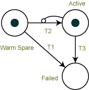
Figure 3: APN model for warm spares
In addition to simply continuing the same process for the same token in a new place wheere it was left off in the old place, the aging allows to account for different pace of aging in a consistent fashion. Let us consider a warm spare scenario that is quite common in reliability: the spare is aging, but at a slower rate than an active component. The corresponding APN model is shown in Figure 3. The source file for this APN model can be found here
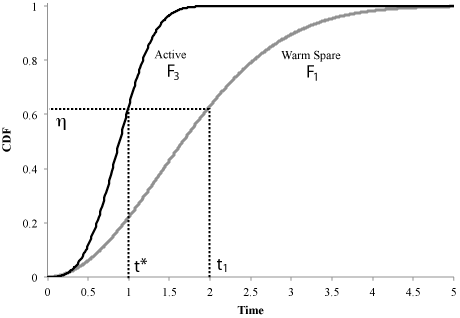
Here T1 is the aging transition for the Warm Spare place, and T2 is an immediate transition (implemented in APN by selecting a fixed transition with a negligible delay, e.g., \(\epsilon=1\times 10^{-6}\)). An inhibitor of multiplicity one disables the T2 transition as long as the token representing the active component is in the Active place. When the active component fails (let us say at time \(t_1 \)), the T2 transition becomes enabled and fires the spare component token into the Active place. The calculation of the corresponding age \(\eta=F_1(t_1)\) and equivalent time \(t^*=F_3^{-1}(\eta)=F_3^{-1}(F_1(t_1))\) are depicted graphically in Figure 4.
Figure 4: Conversion of the equivalent time \(t^*\)
In Figure 4 both \(F_1 \) and \(F_3 \) are Weibull distributions \(F(t)=1-\exp{\left[-(t/\theta)^\beta \right]}\) with the scales \(\theta_1=2, \theta_3=1 \) and shapes \(\beta_1=2, \beta_3=3 \), respectively.
The process of using the aging variable as the current value of the cumulative distribution function is applicable to any distribution and allows muliple jumps from one distribution to another.
One of the attributes of a transition in APN is an age adjustment factor \(a\in \left[0,1\right]\), which multiples the age of a fired token (the transition does not need to be aging). Setting this adjustment factor to zero allows for a renewal of the fired token's age.
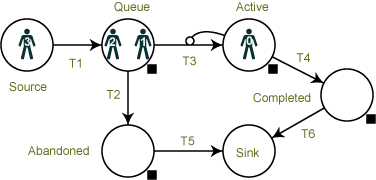
Aging tokens provide a convenient means to enforce different queueing policies. Let us demonstrate how First-in-First-out (FIFO) policy can be implemented. Let us consider a simple queue with abandonment: if a customer does not receive a service after a specified threshold time \(\tau_{max}\), she abandons the queue. The example is selected to emphasize the sensitivity to the selection policy (aggregate statistics are often insensitive to queuing policies). The model is shown in Figure 5. Figure 5: APN model of a queue with abandonment
Here the T1 transition controls the customer's arrival. The number of servers is controlled by the inhibitor for the T3 transition, let us consider a single server, so the inhibitor has multiplicity one. The T2 transition has a fixed delay \(\tau_{max}\). Both arrival (T1) and service (T4) follow exponential distributions. Transitions T5 and T6 have fixed delay \(\epsilon=1\times 10^{-6}\). As a result, customer tokens pause momentarily in the Abandonded or Completed place, respectively. Both places have sensors (denoted in APN with the solid square in the lower right corner) that allow to register each "hit", thus measuring the rates of abandonining or completing the service, respectively. We will also measure the mean number of customers in service and in the queue. In order to implement the FIFO policy we will make the T2 transition aging for the Queue place, and select the age-dependent fixed delay \(\epsilon=1\times 10^{-6}\) for the T3 transition. This will ensure that when the server is free a token that stayed in the Queue place the longest (and therefore has the largest age) is fired first. Individial tokens have their unique IDs displayed (this is an option in APN), so during the animation one can visually track whether FIFO is observed.
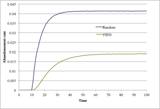
Figure 6: Abandonment rate for FIFO and Random policies, \(\rho=0.8\)
For comparison we also consider a random order for selecting the customers. To implement this policy we can switch off the aging for the Queue place, and select a very fast exponential delay, say \(1/\epsilon=1\times 10^{6}\) for the T3 transition (since T3 is an exponential transition, whether the tokens age or don't does not matter). You can download the source files for the FIFO and random policies, and also the Excel spreadsheet that can control the model parameters for both models (Simply link the XLS file from the parameters menu in APN, and after you linked it once, you can make the changes to the XLS spreadsheet, save it, and then click on the "Update from Linked File" from the parameter menu in APN to automatically update all the model parameters).
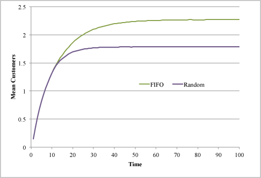
Figure 7: Queue size for FIFO and Random policies, \(\rho=0.8\)
First let us consider a "subcritical" case: \(\lambda=0.8, \mu=1\), so that \(\rho=\lambda/\mu=0.8\) and \(\tau_{max}=10\). Figure 6 shows the benefits of FIFO policy in terms reducing the number of abandoments by more than a half as compared to random. This is expected, since being a "fair" policy, FIFO ensures a more uniform waiting times, while for random policy there will be a larger portion of customers that reach the \(\tau_{max}\) of waiting and leave. There is a penalty, however as observed in Figure 7, as the average time in the queue for FIFO is higher than for random (the \(\tau_{max}\) limit is used more efficiently by FIFO). Here the steady state value of expected queue is 2.27 vs. 1.787 customers for FIFO vs. random policies, respectively. The results reported here are based on ten million replications, with the steady-state value evaluated as the time-average value for the last 10% of the simulation time (simulation time is 100). This might be an acceptable trade-off if the leaving customers are costly.
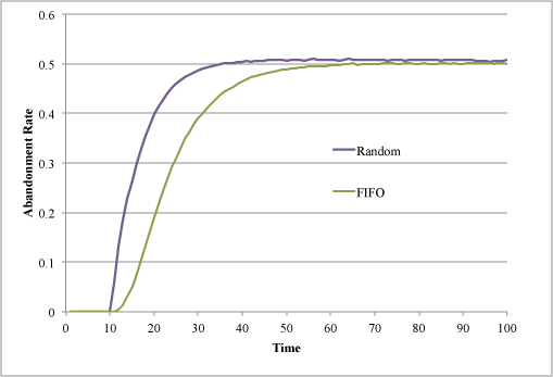
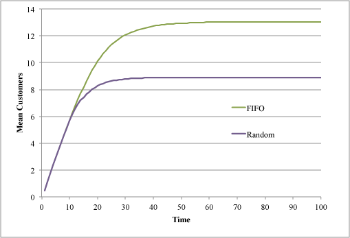
Figure 8: Abandonment rate for FIFO and Random policies, \(\rho=1.5\) Figure 9: Queue size for FIFO and Random policies, \(\rho=1.5\)
It is instructive to consider the same problem in "super-critical" regime where \(\rho>1\) and the system is stable only due to the abandonment effect. Let us consider \(\lambda=\rho=1.5\), while keeping the rest of the parameters the same as before. The simulation time is also the same, but we will use the results from 1 million replications that provide sufficient accuracy here (as compared to the previous example, the number of abandonment is larger, so fewer replications are needed to estimate it). Figure 8 shows the abandonment rates, which are much closer to each other after the warm-up period. In this regime the benefit of FIFO is very small in the long run, while, as seen in Figure 9, the penalty on waiting remains significant (the steady state values are of expected queue is 13.05 vs. 8.911 customers for FIFO vs. random policies, respectively). Effectively, in this scenario the customers wait longer in vain.