
For Complex Systems
(Stochastic) Petri Nets
What are APNs derived from?
Visually, APNs can be considered as a hybrid of Markov chains and Petri nets. Similar to Markov chains, it is a state-space representation where (a finite) number of possible states is represented as circles, and transitions from one state to another are denoted with directed arcs. However, in contrast to Markov chains where states of a system as a whole is modeled, the states of individual entities that comprise the system are modeled instead.
To implement component-based representation, we borrow the notations from Petri nets (a popular tool in computer science) and introduce smaller filled circles (tokens) that represent individual parts of the system and can move between particular larger circles (states) that are referred to as places. There are two advantages to this approach:
- Better scaling properties: a suitable analogy here is arabic/indian numerals: Instead of creating distinct symbol for each number (which is similar to Markov chain idea of representing each state of a system with a separate circle), we use a small number of (10) numerals to code up all the possibilities in a compact fashion (which is similar to tracking behavior of individual components that make up the system). As a result, if we have 10 components and each component can be in 10 states, we will need to have only 100 (rather than 10 billion) states.
- Better visualization of the dynamic of the system, as tokens movements provide important insights into components interactions and the corresponding evolution in time.
How are APNs different from other Petri Nets?
Fundamentlly, in traditional Petri nets (and Stochastic Petri Nets in particular), system components are represented by places. In contrast, in APN components are usually represented by tokens. As a consequence, these tokens are more persistent that their equivalents in SPNs, they have "memory" remembering their past (including their identities). In particular, the state changes in standard Petri nets are interpreted as taking tokens from all incoming places and depositing tokens to the outgoing places. In contrast, APNs merges those two actions into one "movement" of a token from an input place to an output place. As long as tokens are all the same (indistinguishable), both interpretations are equivalent. However, for distinguishable (color) tokens the difference is significant.
In traditional SPNs, transitions represent a separate type of objects that is used to connect places. Transitions are denoted with rectangles, and they serve as transient stops or junctures between the places: in order for a token to move from one place to another it has to pass through a transition. In graph theory the resulting construction is referred to as a bi-partite graph: there are two types of nodes (places and transitions) and links (arcs) always go from one kind of node to the other (an arc cannot go from a place to a place, or from a transition to a transition). There is no restriction on the number of links that can connect the nodes, so a transition can have two (or more) incoming link and only one out going link, which can model merging, or we can have the opposite situation (forking or splitting). This leads to a great modeling flexibility, but this freedom leads to complex routing routes for different colors.
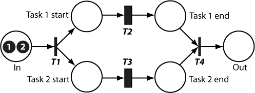
For example, let us consider a common scenario workflow when two activities are executed in parallel for each case.
- Provide a dedicated network to each case. This obviously leads to difficulties in visualization of problems with large number of cases
- Code relatively complex "inscriptions" for the transition that map the tokens colors into specific places. The complexity of the logic here is driven by the fact that enabling of the transition is based not only on an individual input, but rather on the combination of the inputs (only when both incoming branches have tokens of the same color, transition should be enabled)
Effectively, when the tokens are distinguished, transitions serve two distinct roles:
- Represent interactions, such as synchronization, as described in the above example. This interaction is generally symmetric (bi-directional or two-way).
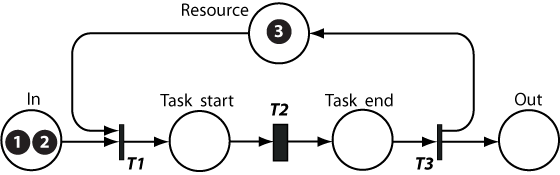
- Route tokens into different places based on their color (for example, divert different classes of customers to different subnets). Usually, this is handled by specifying post conditions based on the place identity. Let us demonstrate this role on the utilization of a resource scenario (see figure "SPN model for utilizing resources"). A standard way to route the colors is to provide a color mapping between the transition and its outputs: so the output for transition T3 is specified based on the differentiation between the types of tokens (so tokens with colors 1 and 2 are moved (fired) into the "Out" place while token a token with color 3 is fired into the "Resource" location). However, if we have different types of resources, say that have color 3 and 4, respectively and it might be important to differentate their utilization (for example if their cost is different), the "local" mapping of colors between a transition and its output places must be more complicated: the output color from transition T1 has to combine all permutations between the resources and the customer types, and the output from T3 must take all these permutations into considerations.
As a result, the lack of limitations on the number of inputs and outputs to a transition leads to the choice between large number of dedicated duplicate subnets or complex inscriptions that take into account complex permutations and must be done programmatically
How APN model interactions among systems' components?
APNs consider default behavior as parallel (independent), and therefore focus on the coupling (interactions) in clearly defined fashion. There are multiple mechanisms that either implicitly or explicitly imply interactions in traditional SPNs. Three of those mechanisms are NOT used in APN:
- Competition for firing from the same place when "single-server" (or limited capacity) policies are used. Single-server policy if the default policy in many versions of SPNs and it provides a compact representation of simple queueing with random order. However, when the tokens are distinguishable, this policy is of limited use, and can be easily represented using the infinite server policy combined with an extra place that only allows one token at a time (by means of an inibitor). The use of infinite server (that effectively assumes token independence) is critical for effective model of complex systems. As a result, to avoid confusion (and lacking standard distinguishing notations with the inifinite server) APN does not use a single-server (or limited capacity).
- Arc multiplicities. In traditional Petri Nets places represent components, with the state space of the component represented by the number of tokens in that place (place marking). There are situations when the state change is a "jump" so that state changes by more than one position. For example, if the old state was represented by five tokens, and the new state by three tokens, this change is represented by the outgoing transition of multiplicity two that fires two tokens simultaneously. In contrast, in APNs the main mechanism for representing system components is tokens, and they interact with transitions individually: if a place has several tokens in a place with an outgoing transition, each token has its clock with respect to the transition. The state of the token can be represented by its integer attribute (color), and upon firing through a transition we can specify the increment to that color (so if the color was five, this increment can be set to -2, resulting in the token of color three). Alternatively, if one desires to coordinate the firing of tokens - and fire two tokens at the same time, this can be modeled by providing an explicit construction with an inhibitor that allows only two tokens in a place at a time.
- Marking dependence is effectively a "catch-all" means to capture system interactions that are not captured otherwise. There is no standard graphical notations, so the dependence cannot be captured visually. This is fundamentally a programmatic way of capturing the dependence, and it is avoided in APN.
Instead there are are specific mechanisms for modeling two types of interactions:
- One-way interactions: Component A influences behavior of B (but not the other way around). Triggers Triggers, which are either inhibitors or enablers (the inhibitors' opposites) are used for this purpose.
- Two-way (symmetric) interactions (coordination) - Merging Joints are used for this purpose. Which can be considered as specific subset of immediate transitions in traditional SPNs designed specifically to simplify coordination of token movements.
Routing role is considered to be separate from interaction, as the routing concerns individual tokens. So in APNs transitions (directed arcs) can link place nodes directly, similar to state space diagrams for Markov chains, and those transition can have color-specific policies, thus serving the routing role as well.
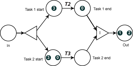
Let us show how the challenges of coordination are handled as a result. First we look at the execution of two tasks in parallel for several cases. The resulting model is shown in the figure "APN model for two parallel tasks" and one can see that the logic of the model simply mimics the idealized SPN models with joints serving the splitting and merging role, and the transitions T2 and T3 depicted using directed arcs (without separate transition nodes). The merging joint has policy "I" (see Merging Joints) that ensures that only tokens with the same ID are merged. APN provides an option to use IDs as visualized token labels, as shown in the figure.
The second scenario with handling the resources is inherently more complex. We will show here a specific solution that implies that the duration of the task is independent on the type of utilized resources (but can depend on the type of customer). An alternative model where the resource does impact the task duration is also possible. The model is certainly more complex than the idealized version for SPN (see Figure "SPN model for two parallel tasks"). However, the SPN model is only valid for a non-distinguishable resources, unless complex inscriptions are utilized. Otherwise, each resource requires a dedicated subnet that are fused together in the shared pool place.
APN model is organized as follows. When a case token appears in the "In" place it is duplicated first. One of the copies is used to initiate the resource request. If the resource is available, the merging joint is fired, and the merged token is deposited into the "Resource seized" place. The resulting token inherits resource properties (this is ensured by selecting as dominant the upper input branch into the joint, as visualized by the thicker line of the dominant arc). The ID from the task token is inherited as a shadow or recessive ID for the token (it will be used later). The joint type is "Any" as here no requirement to the type of resource is specified. This model can be further refined if only some of the resources are suitable for the task (in this case colored policy can be selected for the joint). The resulting token is duplicated next to keep a resource copy. The other copy is merged with the copy of the task token, where the recessive ID merging option "R" is utilized (since the recessive or shadow ID of that token matches the task's ID). After the task is completed and the token moves to the "Task end" place it gets duplicated with one copy used to indicate the completion of the task (the "Out" place), while the other copy is used to merge with the copy of the resource and release the resource. Here the dominant input is from the "Resource copy" place, and "R" matching policy is utilized.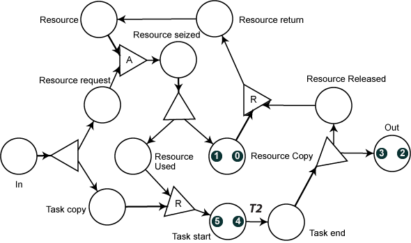
How is APN different from other Discrete Event Simulations?
There are some similarities to the standard process-interaction DES (such as Arena), as places resemble the "servers" (process blocks), and token resemble transient entities (transactions). In addition, the split joint is similar to the Duplicate block, and the merging joint is similar to Batch block. However there are important differences as well:- Initialization: in APN tokens can be directly put in the appropriate places without the need to generate them first and route to the proper initial place. This makes models more compact and eliminates significant overhead during simulation.
- APN allows for direct modeling of a "race" (deferred choice): several processes can occur to the same entity at the same time (no need to create a duplicate and route it through the separate process, then retrieve the entity from the original process).
- Standard DES have no triggers: there is no accepted standard means for modeling asymmetric (one-way) interactions. State-space representation is often used to model availability of resources, but this state space is not visually connected to the main model.
V.Volovoi "Abridged Petri Nets", ArXiv: 1312.2865 [cs.OH](2013);. The current version of the paper is here.
Aging Tokens present another distinguishing feature of this SPN extension, as they provide a compact means to model transition rates that are time-dependent. Effectively "age" of a token is a continuous label with the value from [0,1]. The value of this label can be affected in a continuous fashion as the token stays in the same place, or in a discrete fashion upon firing of a transition. The concept of "aging" corresponds to the former. However, transitions can be either aging or not. In the current version, each place can be an input to no more than one aging transition. If there are no aging transitions, tokens don't age (that is, their ages remain unchanged). There can be more that one transition for a given place that will affect the age in a discrete fashion (there is no conflict, since this effect is realized only when firing occurs). These concepts were first introduced in the following paper:
V.V. Volovoi, “Modeling of System Reliability Using Petri Nets with Aging Tokens,” Reliability Engineering and System Safety, 84, no. 2 (2004): 149–161(PDF)